Falling Loop Model
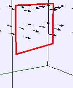
The EJS Falling Loop Model
shows a
conducting loop falling out of a region of uniform magnetic field.
It also plots the velocity of the loop as a function of time. Users
can change the size the the loop, the orientation of the loop to the
field, the size of the field and the location of the loop and field.
Users can examine and change the model
if they have Ejs installed.
Exercises:
- Run the simulation. The
arrows show the uniform magnetic field. A conducting loop falls under
the influence of gravity, but it also experiences a force as it goes
from a region of no magnetic field to a constant magnetic field. What
is causing this upward force? (Hint:
There is an induced current in the loop. Why? This means there is a
magnetic force in what direction(s) on the side(s) of the loop?)
- Move the loop up and the field down so that the loop falls freely
before entering the field. Describe your observations of the loop and
the velocity versus time plot.
- Reset the simulation. Observe the plot of the velocity versus
time. How can you tell from looking at the plot that the force on the
loop is non-constant for part of the fall? Once the loop is completely
out of the field, the force is constant. Why? What is the acceleration?
- Run the simulation again,
but this time set the angle to ± 90o.
Explain what
you observe. Why does the angle matter?
- When
something is falling
and its velocity stays the same, it is
said to have reached terminal velocity. Reset the simulation and make
sure that the angle between the loop and field is 0o (this
is the angle between
the surface
of the loop and the field). Click on the wrench
button below the velocity
plot to open up DataTool
(a data analysis tool). For your set-up,
does the velocity seem to level off for part of the fall? If so, this
is the terminal velocity of the
loop as it is falling through the
field. If not, change the size of the loop and run it again to get a
terminal velocity. Record this value and along with the size of the
loop. Run it
again with different loop sizes. How does the terminal velocity depend
on the loop height (size in the vertical direction)?
- Run the
simulation with the
loop starting at the top of the
simulation window but completely within the magnetic field (you may
need to make the loop smaller or the field extent larger so the loops
stays within the field for several time steps). What is the
acceleration of the loop while it is
completely in the magnetic field. Why? Explain the plot you
get for this motion (specifically, the linear and non-linear
parts)?
- When the loop has reached
terminal velocity, the
acceleration due to gravity is just balanced by the acceleration due to
the magnetic forces on the loop. (Why?) Show that, with an angle of 0o,
the terminal velocity is given by gmR/(B2l2)
where g
is the acceleration due to
gravity, m
is the mass of the
loop, R
is the resistance of
the loop, B
is the magnetic
field, and l
is the length of
the side that you can't adjust. Given the following values, what is the
magnetic field in this simulation? m
= .001 kg; R
= 0.1 Ω, l
= 0.1 m and, of course, g
= 9.8 m/s2.
Note that the plot gives you velocity in cm/s.
- With your data showing in
the DataTool,
if you click-drag your mouse over a section of the plot, you can
highlight that section and Fit
it. From the fit, double-check that the free-fall acceleration
is what you expect (the
units of the velocity are in cm/s).
- Data Analysis:
Reset the simulation so that the loop's initial velocity is zero and it
will begin by falling out of the field (non-constant acceleration as it
begins its decent). With DataTool,
try fiting the region of the curve for non-constant acceleration
(make sure the Fit
checkbox is checked).
Because is it asymptotically reaching a constant velocity (terminal
velocity), you will need to input your
own equation. Select the region of the plot where the
loop is experiencing a magnetic force. Double-click in the box showing
the equation for a line and Fit
Builder will open.
Input the following equation for Line1: -a*(1-exp(-b*t)).
Now, AutoFit
the data to your newly defined Line1
and record the parameters a
and b.
As t
gets very
large in the equation for Fit1,
show
that Fit1
(=velocity) is equal to -a.
Therefore, check that a
is close
to the terminal velocity (the units of velocity
are in cm/s). Similarly, since the analytic expression for
a particle with drag is v(t) = -vt(1-e-(g/vt)t)
where vt
is the terminal velocity, compare b
to g/vt.
References:
- Giancoli, Physics
for Scientists and Engineers,
4th
edition, Chapter 29
(2008).
Credits:
The Falling Loop Model was created by Wolfgang Christian and Anne J
Cox
using the Easy Java Simulations (EJS) authoring and modeling
tool. The exercises are by Anne J Cox.
You can examine and modify a
compiled EJS model if you run the
program by double clicking on the model's jar file.
Right-click
within the running program and select "Open EJS Model" from the pop-up
menu to copy the model's XML description into EJS. You must,
of
course, have EJS installed on your computer.
Information about EJS is
available at: <http://www.um.es/fem/Ejs/>
and in the OSP ComPADRE collection <http://www.compadre.org/OSP/>.